.png)


In a previous blog, I broke down the various different storage modes and connectivity types such as Import, DirectQuery, Live Connection, Mixed mode and Direct Lake. You can read this here: Power BI Storage Modes Demystified. The goal of that blog was to showcase the various ways to ingest and establish a connection and the core differences between them all.
This blog is more focused, as rather than comparing Direct Lake to everything else again, the purpose here is to properly unpack Direct Lake itself. Direct Lake gets mentioned a lot in Fabric conversations, but it is often explained at a very high level and I have been meaning to write this deeper dive. Usually, it gets positioned as the best of both worlds. So, the performance characteristics of Import, the freshness benefits associated with DirectQuery, without the need of refreshing the data. That is a useful and fair starting point, but it has also led people to jump to conclusions, such as assuming Import and DirectQuery are dead or that Direct Lake will always be faster than Import.
What is Direct Lake actually doing under the hood? Where is the data really being read from? Why can the first query feel different from the next? What is framing? Why does the underlying Delta table design matter? What is Direct Lake on OneLake and Direct Lake on SQL, and what are the differences?
That is what this blog is here to cover. So, let’s start with the foundation of where the data actually lives in a Direct Lake setup.
One thing worth calling out before we get into it... Direct Lake requires a Fabric capacity licence. If you want the full licensing picture, we have a detailed guide on that here: Navigating Power BI & MS Fabric Licensing.
Where the data actually lives in Direct Lake
To understand Direct Lake properly, the first thing to get clear on is where the data actually sits, and just as importantly, what Fabric items it covers.
With the classic Import storage mode, which is available across all data source types, Power BI takes a physical copy of the data and stores it inside the semantic model. Import was always (and I believe, still is) the most used and common connectivity type. Direct Lake is different! The data remains in Microsoft Fabric, with the underlying data backed by Delta tables in OneLake. In practice, many people first associate this with Lakehouses and Warehouses, and that is fair and true. For a deep dive difference between Lakehouses and Warehouses, check out blog here. But Microsoft’s guidance has widened that conversation, referring to Direct Lake working with tables from Fabric data sources backed by Delta tables. That is important, from my own usage I have not just used Direct Lake against Lakehouses and Warehouses, but also against a mirrored database and a SQL database in Fabric. If you want to understand mirroring (and Shortcuts) more, I covered that here.
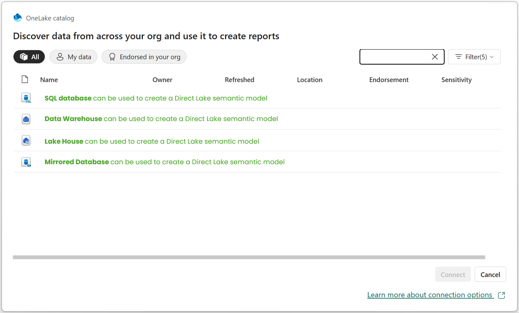
In the image above, I simply wanted to illustrate that Direct Lake is not tied to just one Fabric item type. It can work with different Fabric items, such as the ones shown above but not limited to those. Again, it comes back to Delta tables.
With the above said, there is an important distinction between two types of Direct Lake. We have, Direct Lake on OneLake and Direct Lake on SQL (confusing, right?!). Now, I do not want to overcomplicate this too early, so I will simply raise that here and we will come back to it properly later in the blog. So do not worry if you don't understand the differences, right now, we will come back to this.
The key point for now is that the data is still living in OneLake. Once you understand that, a lot of the wider Direct Lake conversation starts to make more sense. It helps explain why Direct Lake feels different to Import, why Fabric becomes such an important part of the picture and why terms like framing, transcoding and fallback start to come into the conversation.
So before getting into performance, query behaviour or anything else, it is worth grounding this point clearly. In a Direct Lake approach, your starting point is a Fabric data source backed by Delta tables in OneLake. On top of that, you have a semantic model and then on top of that sits your report. In other words, the report is not querying some completely separate imported copy hidden away inside the model in the same way many Power BI users are used to thinking about it.
How a Direct Lake semantic model gets created from a Fabric item
Now that we have covered where the data actually lives, the next useful question is a practical one. How do you actually start creating a Direct Lake semantic model?
This is where the experience has evolved a bit and I will have a separate blog on the differences in the development experience (traditional PBI Dev vs New MS Fabric Dev). At the start, this felt much more like a Service-first experience inside the Microsoft Power BI Service. But today, you can also work with Direct Lake semantic models from Power BI Desktop, which is an important shift for people who are more used to the Desktop development experience we always had.

Starting in the Service is very straightforward. In the screenshot above, I am inside my Gold Warehouse in Fabric called "WH_QuickBooks_Gold" and we can create a new semantic model directly from that Fabric item. Notice, in the green box you can select "New semantic model". That is already a notable difference from the older approach many Power BI users are used to, where the starting point would typically be Power BI Desktop.
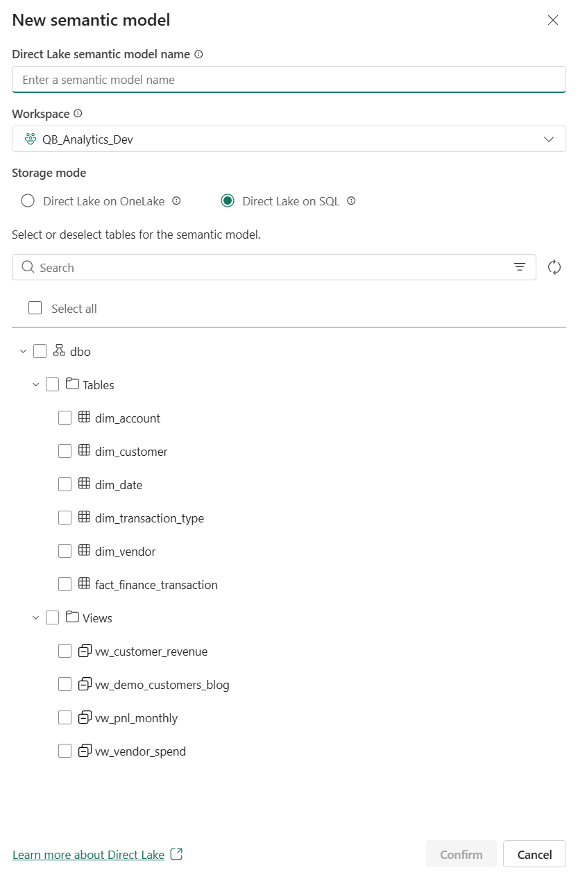
Once you do that, Fabric gives you the option to choose the Direct Lake type, as we mentioned above. In this case, you can see the two types available which are Direct Lake on OneLake and Direct Lake on SQL. Again, I do not want to go too deep into that distinction just yet, as there is a later section dedicated to it, but it is useful to see here that this decision can appear at model creation time.
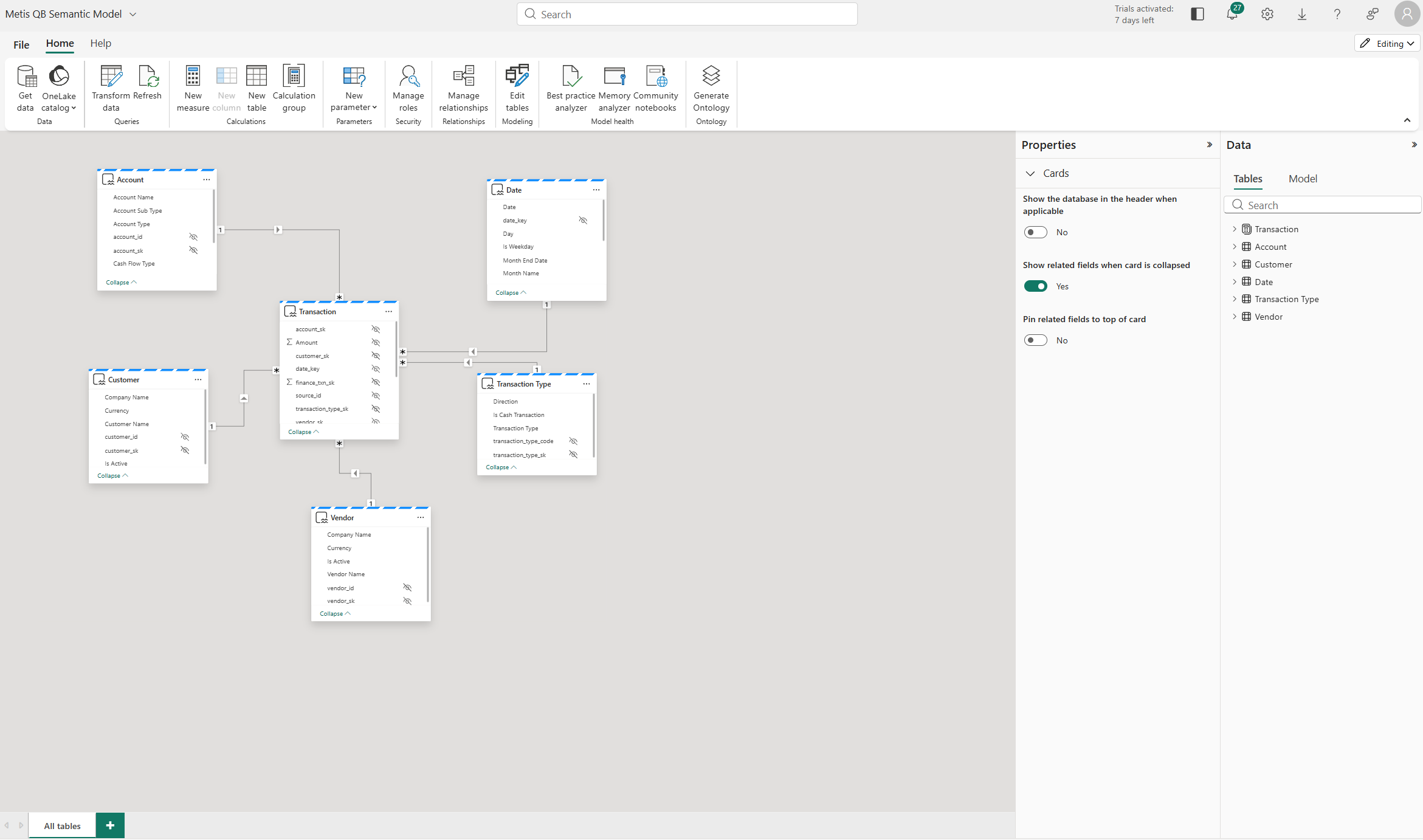
After creation, the semantic model can then be opened and worked on directly in the Service itself and this is what you are seeing in the screenshot above. That means the experience is not just about creating the model online, but also about being able to shape and maintain it there as well. Again, this reinforces the point that the starting point is the Fabric item, with the semantic model sitting over it.
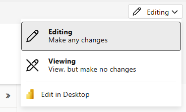
What is also important now is that the experience does not stop in the Service. You can move from the online experience into Power BI Desktop, which matters because many of us are still far more familiar and comfortable working there. So as you can see above, you can click through whilst in the Power BI Service to a "Edit in Desktop" button.
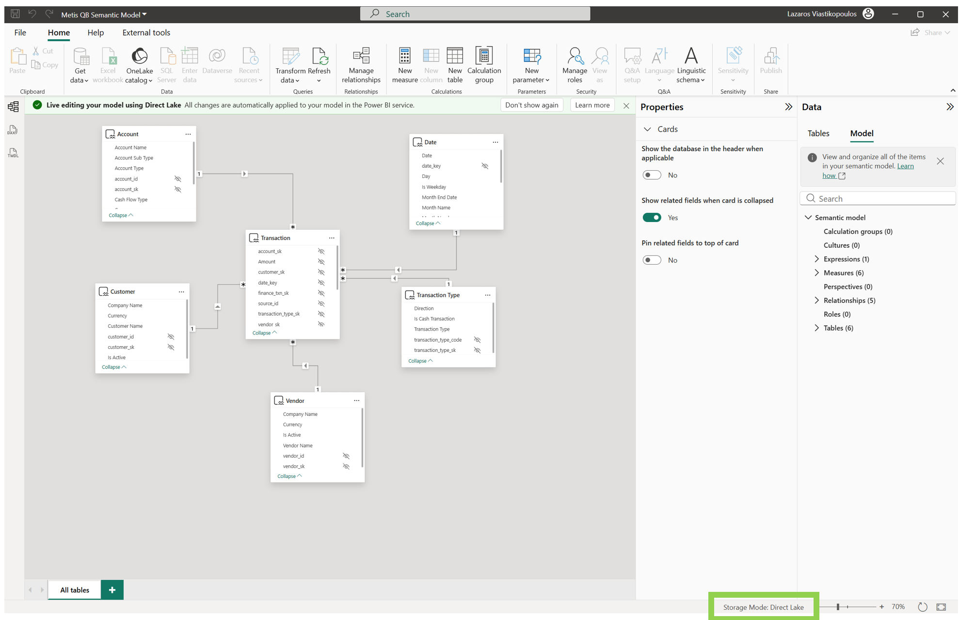
Once in Power BI Desktop, you can continue working with that same Direct Lake semantic model there too. In the example above, you can see the model opened in Desktop, with live editing for the Direct Lake model - see the green banner labelled "Live editing your model using Direct Lake...". So, the creation and modelling experience is no longer confined to the Service only. From memory, when Direct Lake was first introduced it was not possible to edit your model from Power BI Desktop, but as you can see we now can.
So, we can see above that our Direct Lake journey can begin from two places: directly inside the Microsoft Fabric/Power BI Service or through Power BI Desktop. That is important, because it makes Direct Lake feel much less like a niche Service-only path and much more like part of the wider Power BI modelling experience.
One additional point worth calling out, if you are a long-time Power BI user and you go through this experience in Power BI Desktop, it can feel a little odd at first. It was for me! You still have the modelling side there, but the reporting element almost feels like it has disappeared. It is one of those moments where you open Desktop and think, hold on, where has the other half gone?
Why Direct Lake is not classic Import refresh
Now, it is very easy to think of Direct Lake simply as being like Import, but better. Faster, newer, more modern, but still basically the same idea underneath. But, that is not really the right way to think about it.
With the Import storage mode, Power BI takes a physical copy of the data and stores it inside the semantic model. When you refresh it, that imported copy is what gets refreshed. That is the way most Power BI users have been used to thinking about it for years.
Direct Lake is different though. Yes, it can deliver very strong performance, but the way it reflects source changes is different from the traditional Import approach. The data is still sitting in Fabric and the semantic model is working over that Fabric data rather than maintaining its own traditional imported copy in the same way.
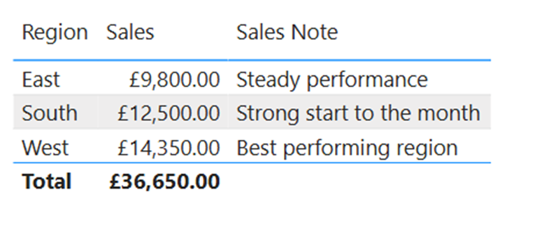
The screenshot below shows a demo report before I apply any source changes. Focus on the South region row. At this point, Sales are £12,500 and the Sales Note is “Strong start to the month”. That is our starting position.
This matters because if you go into Direct Lake assuming refresh works exactly like classic Import, you will end up misunderstanding what is actually happening behind the scenes. Direct Lake introduces concepts that do not really belong to the classic Import conversation in the same way, such as framing, automatic updates, column loading, and in some scenarios even fallback.
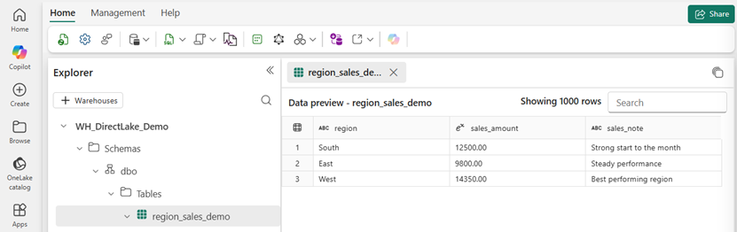
In the screenshot below, we can see the underlying Fabric table in the Data Warehouse before any changes. This is the source for the report above. Again, look at the South row. You can see the same values sitting in the Warehouse such as a sales amount of £12,500 and the Sales Note is “Strong start to the month”. This is important because it ties the report result back to the source data in Fabric.
A simple way to see this is to make a change in the underlying Fabric table and then observe what happens in the report. That is the kind of moment where the Import approach starts to break a bit. You are no longer just thinking in terms of "Power BI has its own copy and I need to refresh that copy". The relationship between the model and the source is different enough that Direct Lake needs to be understood on its own terms.
Previously as in before Direct Lake (and still without Fabric capacity), handling very large models in Power BI often meant Mixed mode (Composite Models) combining Import and DirectQuery, building aggregation tables, setting Dual storage mode correctly and carefully managing what sat where. It worked, but it required good thought and overhead. Direct Lake changes that conversation significantly.
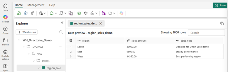
In the next screenshot, we can see the same Warehouse table after the update I made with a SQL query. Still looking at the South row, the values have now changed to sales to £20,000 and sales note to "Updated for Direct Lake demo". In other words, the source in Fabric changed first. Here is the very important point, I did NOT run a model refresh here. The source data in Fabric was updated, and the Direct Lake semantic model picked up that change, which then flowed through to the report. That is exactly why it is not right to think about Direct Lake as a like for like Import refresh but with a newer label.
Now, I am not saying there is no refresh behaviour involved at all. What I am saying is that it is not helpful to mentally categorise Direct Lake under the same bucket as Import and leave it there. That oversimplifies it too much.
The screenshot below now brings us back to the report after the source update. Once again, focus on the South row. The visual now reflects the new values. We have £20,000 and "Updated for Direct Lake demo". That is the practical setup for the next part of the conversation, because this is where we start moving away from the classic Import way of thinking and into concepts like framing.

So the key point in this section is simple. Direct Lake should not be treated as just a better version of Import refresh. It is a different approach, and if you want to understand why it behaves the way it does, you need to start moving into concepts like framing, which is what we will explore next.
One last point, Import mode uses the VertiPaq engine under the hood, which is where a lot of Power BI’s performance comes from. VertiPaq is a columnar engine built for high compression and fast analytical queries. Direct Lake uses the VertiPaq engine for query processing too, which is one of the main reasons it can perform so well. Now, you do not need to understand every moving part to use Power BI well. In the same way you can drive a car without knowing how the engine works, you can build in Power BI without knowing every internal detail. But if you do want to understand the VertiPaq engine more deeply, especially in the context of Import mode and the different encoding types, I have covered that in another blog as well.
What framing actually is
So, continuing from above, if I did not run a model refresh, what actually happened? Well, this is where framing comes in.
With Import mode, we are used to the idea that the semantic model holds a physical copy of the data and when we refresh, we refresh the entire data (unless we have incremental refresh configured - which if you want to learn about check out this blog here). As I said previously, Direct Lake is different! Microsoft describes framing as a Direct Lake operation triggered by a semantic model refresh, but unlike a standard Import refresh, it is typically a lower cost metadata operation that can take only a few seconds. Rather than rebuilding a full imported copy of the data, the semantic model analyses the metadata of the latest version of the Delta tables and updates its references to the latest files in OneLake.
To make that a bit more clear, it is worth looking at the Lakehouse side. In the screenshot below, I clicked "View files" on an individual Lakehouse table to show the underlying Delta structure.
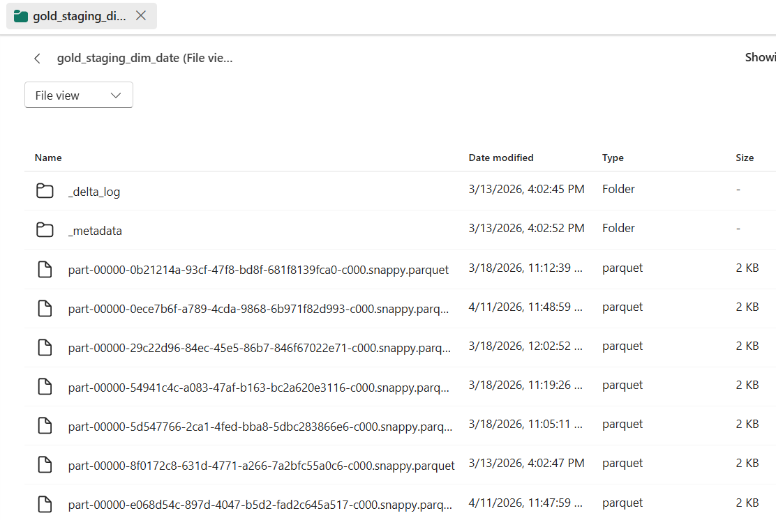
Notice, Fabric data is stored in Delta format, which means data files plus a transaction log. Microsoft’s Warehouse documentation also states that Warehouse data is stored in Delta tables, which are Parquet data files with a file-based transaction log. So when we talk about framing, this is part of what we are really talking about... the semantic model aligning itself to the latest valid state of those Delta tables in OneLake.
Now, in the screenshot below, we can see the semantic model setting "Keep your Direct Lake data up to date" turned on. This allows Power BI to detect changes in OneLake and automatically update the Direct Lake tables included in the semantic model. It is also worth noting that the standard scheduled refresh option is turned off below it, which helps show that this is not the same pattern as a traditional Import refresh.

In the previous section, I updated the source table and the report later reflected that change without me running a standard model refresh. Framing is one of the key reasons that behaviour starts to make sense. This setting is there for a reason. In some cases, the default automatic behaviour will be fine. In others, you may want tighter control so it lines up with your ETL process, in which case you can disable it and manage when those updates happen yourself.
The important nuance here is that framing sets a point in time for what the Direct Lake semantic model sees. In other words, Direct Lake queries return data based on the state of the Delta table at the point of the most recent successful framing operation, which is not necessarily the absolute latest state of the Delta table at every possible moment. That is a very different idea from the simpler "refresh the imported copy" way many of us are used to.
Another useful way to think about it is this: framing is not the same thing as loading all of the data into memory. It is the step where the semantic model updates its understanding of the latest valid Delta table state in OneLake. Then, when a query is actually run, Direct Lake loads the required columns into memory if they are not already there.
So, framing is not just another name for Import refresh. It is one of the core Direct Lake operations that keeps the semantic model aligned to the latest valid Delta table state in OneLake, without behaving like a standard Import refresh.
What column loading means in Direct Lake
Now that we have covered framing, the next part to understand is column loading, which Microsoft also refers to as transcoding. In the past, I have also referred to this as paging, and if you have seen me use that term before, this is the same general idea. Microsoft explains that Direct Lake semantic models only load data from OneLake as and when columns are queried for the first time. So, unlike Import mode, Direct Lake is not pulling all model data into memory upfront so you can see how this can be more efficient. Instead, it works out what is needed for the query, checks whether those columns are already in memory and if not, loads them from OneLake. Side note... this reminds me a bit of the older Premium Gen1 days, where memory pressure and eviction were real things to think about. It is not the exact same, but the idea of memory being shared and data being brought in and pushed out when needed does feel familiar.
This is where some of the older wording around paging came from. As a practical way of thinking about it, it still helps, because data is being brought into memory only when needed. But if I want to stay closer to Microsoft’s current wording, column loading or transcoding is the better term. Microsoft still uses the language of data being paged in and out of memory in some Direct Lake guidance, but column loading is the clearer term to use now.
The key point is what happens when a DAX query hits the semantic model. Direct Lake first works out which columns are needed to answer that query. That includes columns directly referenced in the query, but also columns needed because of relationships or measures which makes total sense. In reality, that usually ends up being a much smaller subset than all the columns in the model because if it weren't it would not be as efficient. If any of those required columns are not already resident in memory, Direct Lake loads the full data for those columns from OneLake. Reading through the Microsoft guidance, this is typically a fast operation, but it can depend on things like column cardinality.
Now, once those columns are in memory, they become resident. That matters, because future queries that only need those same resident columns do not need to load them again. This is one of the reasons Direct Lake starts to make more sense once you stop thinking about it through the usual Import lens. It is not loading everything up front. It is loading what it needs, when it needs it. I think that is important to repeat... It is loading what it needs, when it needs it.
One extra way to make this more tangible is to actually check which columns are resident in memory. In the screenshot below, I used DAX Studio and specifically the DISCOVER_STORAGE_TABLE_COLUMN_SEGMENTS DMV. I do not want to turn this into a deep dive here, but it is a very useful way to look under the hood.
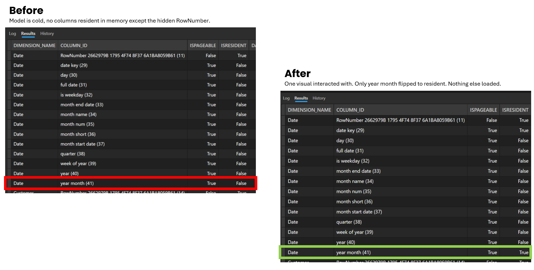
The key column to focus on is ISRESIDENT. In the Before view, the model is cold, so apart from the hidden RowNumber, nothing is resident in memory yet. You can see that Year Month is there, but ISRESIDENT is set to False. I then ran a very simple report using just Year Month with a measure. In the After view, Year Month has now flipped to ISRESIDENT = True, which shows that the column has now been loaded into memory. That is a simple but very useful way to see column loading in action. I do not want to go too far down the rabbit hole here, but if you want to understand this area more deeply, Chris Webb has a great set of blogs on it, so be sure to check those out here.
It is also worth knowing that once a column is loaded into memory, it does not stay there forever. Microsoft says a resident column can later be removed, or evicted, for a few reasons. That could be because the model or table was refreshed after a Delta table update at the source, because the column has not been used for some time or because there is memory pressure on the capacity. Microsoft also refers to excessive paging in and out of Direct Lake model data when memory pressure becomes a factor.
So, the key point here is fairly straightforward. After framing has aligned the semantic model to the latest valid state of the Delta tables, column loading is what happens when a query actually needs data. Direct Lake loads the required columns from OneLake, keeps those columns resident in memory for later use and may evict them later if needed. That is one of the reasons Direct Lake can be memory-efficient while still using the VertiPaq engine for query processing.
There are two Direct Lake types: OneLake and SQL
Above in the blog, I briefly called out that there are two types of Direct Lake and said I would come back to it properly. Well, this is that point. At a high level, we now have Direct Lake on OneLake and Direct Lake on SQL.
I am still playing around with these myself, but the easiest way to think about it is this. Direct Lake on OneLake is the OneLake-first option. Microsoft says it is not connected to the SQL endpoint, it supports tighter integration with OneLake features such as OneLake security and it can produce more efficient DAX query plans because it does not need to perform checks for SQL-based security. It is also the option that supports bringing together tables from multiple Fabric data sources backed by Delta tables, which I can see how it can be useful.
Direct Lake on SQL is different though, and worth calling out what we had from the beginning. This is the option tied to the SQL analytics endpoint of a Lakehouse or a Warehouse. In other words, the SQL endpoint is part of the picture here and that has knock-on effects. Microsoft says this option can use the SQL endpoint in ways that Direct Lake on OneLake does not, which is why some behaviours and limitations start to diverge between the two.
This is also why the distinction matters more than it might seem at first. When someone says "I am using Direct Lake" that is no longer quite enough on its own. Are they talking about the OneLake or the SQL option? Because the answer affects things like security behaviour, source flexibility and whether DirectQuery fallback is even part of the conversation at all, which we will explore in the below section.
As I said, I am still exploring this and will have more on it soon, but be sure to also check out Microsoft’s own comparison. They have a useful table that breaks down the differences between Direct Lake on OneLake and Direct Lake on SQL here.
The key takeaway here is that we now have Direct Lake on OneLake and Direct Lake on SQL, and separating those two makes the rest of Direct Lake much easier to understand, especially when we get into fallback next.
What is Fallback in Direct Lake?
As this is a Direct Lake blog, it only makes sense to also cover Fallback or Direct Query Fallback. It's also helpful that we first explained the differences between Direct Lake on OneLake and Direct Lake on SQL in the above section, as the fallback conversation becomes easier to make sense of.
So, if you have not come across this before, it basically means a query stops being handled in Direct Lake mode and falls back to Direct Query instead. Hence, fallback. Also do remember, Direct Query is one of the slowest connectivity types. Now, this happens when Power BI cannot keep that query within the constraints of Direct Lake mode. In that situation, the table no longer operates in Direct Lake mode for that query and the data is retrieved directly from the SQL analytics endpoint of the Lakehouse or the Warehouse.
From those types we mentioned, Direct Query fallback only applies to Direct Lake on SQL. It does not apply to Direct Lake on OneLake. Microsoft gives some clear examples of where this can happen. One is when the semantic model is querying a view in the SQL analytics endpoint. Another is when it is querying a table in the SQL analytics endpoint with row-level security (RLS) applied. Microsoft also says fallback can happen when a Delta table exceeds the capacity guardrails which you can see here. So this is not some super rare theory as there are specific situations where Direct Lake cannot stay in Direct Lake mode.
One interesting nuance worth calling out is freshness. When fallback happens, the query is not bound by the last framing operation. Microsoft says those fallback queries return the latest data because they go straight to the SQL endpoint. So in that moment, you are not getting Direct Lake behaviour. You are getting DirectQuery behaviour, with all the trade-offs that brings.
Microsoft is also pretty clear that fallback is not something you should be comfortable relying on and I personally agree with this. If possible, design your solution and size your capacity to avoid it, because it can lead to slower query performance. Fallback is a safety net, not the target.
Summary
If you made it this far, you now have a much more complete picture of what Direct Lake is actually doing under the hood, which was the whole point of this blog.
The short version is this. Direct Lake is not Import with a new label. The data lives in OneLake, backed by Delta tables. Framing keeps the semantic model aligned to the latest valid state of those tables. Column loading (transcoding) means only the columns a query actually needs get pulled into memory, not everything up front. There are now two options, Direct Lake on OneLake and Direct Lake on SQL, and they are not identical. Also, we have fallback, which only applies to the SQL type and is a safety net you should be designing to avoid rather than relying on. I will keep adding to this as I build more with it myself. There is still more to cover, including a deeper look at the two Direct Lake types and how the development experience differs from the traditional Power BI Desktop workflow. If you found this useful, share it with someone who is just getting started with Fabric. And as always, if something here is wrong or has changed, let me know.


.png)
.png)
%20(8).png)